Feature Visualization
Hint
Author: Qingmei Tang
Proof: Yifan Feng (丰一帆)
Basic Usages
DHG provides an interface to visualize the distribution of features:
Input the features and label (optional);
Specify parameters (i.e., the dimensionality of the visualisation, point size, color and the method of dimensionality reduction);
Call
plt.show()function to show the figure/animation.
Note
The plt is short for matplotlib.pyplot module.
Visualization of Features in Euclidean Space
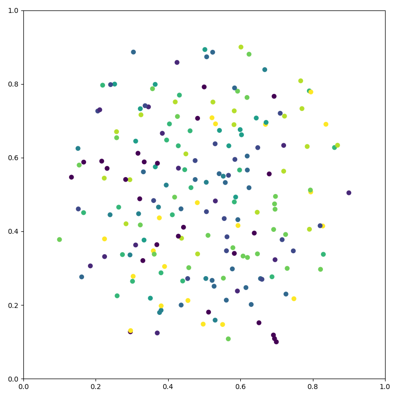
>>> import dhg
>>> import numpy as np
>>> import matplotlib.pyplot as plt
>>> import dhg.visualization as vis
>>> lbl = (np.random.rand(200)*10).astype(int)
>>> ft = dhg.random.normal_features(lbl)
>>> vis.draw_in_euclidean_space(ft, lbl)
>>> plt.show()
Visualization of Features in Poincare Space
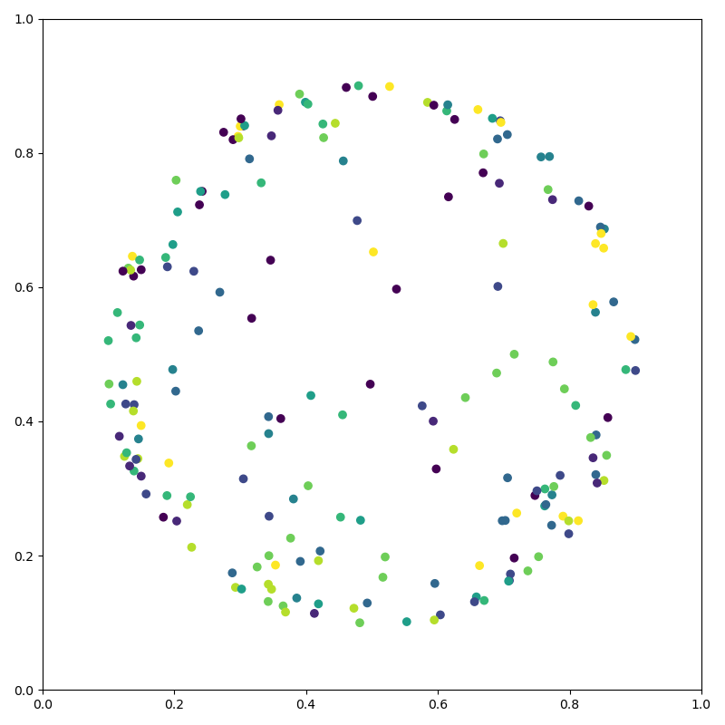
>>> import dhg
>>> import numpy as np
>>> import matplotlib.pyplot as plt
>>> import dhg.visualization as vis
>>> lbl = (np.random.rand(200)*10).astype(int)
>>> ft = dhg.random.normal_features(lbl)
>>> vis.draw_in_poincare_space(ft, lbl)
>>> plt.show()
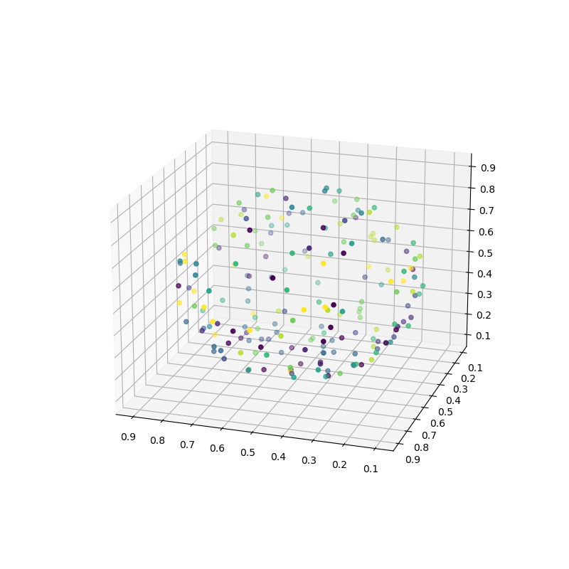
Make Animation
We provide functions to make 3D rotation animation for feature visualization.
Rotating Visualization of Features in Euclidean Space

>>> import dhg
>>> import numpy as np
>>> import matplotlib.pyplot as plt
>>> import dhg.visualization as vis
>>> lbl = (np.random.rand(200)*10).astype(int)
>>> ft = dhg.random.normal_features(lbl)
>>> vis.animation_of_3d_euclidean_space(ft, lbl)
>>> plt.show()
Rotating Visualization of Features in Poincare Space
>>> import dhg
>>> import numpy as np
>>> import matplotlib.pyplot as plt
>>> import dhg.visualization as vis
>>> lbl = (np.random.rand(200)*10).astype(int)
>>> ft = dhg.random.normal_features(lbl)
>>> vis.animation_of_3d_poincare_ball(ft, lbl)
>>> plt.show()
Mathematical Principles of Hyperbolic Space
The hyperbolic space is a manifold with constant Gaussian constant negative curvature everywhere, which has several models. We base our work on the Poincaré ball model for its well-suited for gradient-based optimization.
The Poincaré ball model with constant negative curvature \(-1 / k(k>0)\) corresponds to the Riemannian manifold \(\left(\mathbb{P}^{n,k}, g_{\mathbf{x}}^{\mathbb{P}}\right)\). \(\mathbb{P}^{n,k} = \left\{\mathbf{x} \in \mathbb{R}^{n}: \| \mathbf{x}\|<1 \right\}\) is an open \(n\)-demensionsional unit ball, where \(\|. \|\) denotes the Euclidean norm. Its metric tensor is \(g_{\mathbf{x}}^{\mathbb{P}} = \lambda_{\mathbf{x}}^{2} g^{E}\), where \(\lambda_{\mathbf{x}} = \frac{2} {1- k\|\mathbf{x}\|^{2} }\) is the conformal factor and \(g^{E}=\mathbf{I}_{n}\) is the Euclidean metric tensor. For two points \(\mathbf{x}, \mathbf{y} \in \mathbb{P}^{n,k}\), we ues the Möbius addition \(\oplus\) operate adding by connecting the gyrospace framework with Riemannian geometry:
The distance between two points \(\mathbf{x}, \mathbf{y} \in \mathbb{P}^{n,k}\) is calculated by integration of the metric tensor, which is given as:
Denote point \(\mathbf{z} \in \mathcal{T}_{\mathrm{x}} \mathbb{P}^{n,k}\) the tangent (Euclidean) space centered at any point \(\mathbf{x}\) in the hyperbolic space. For the tangent vector \(\mathbf{z} \neq \mathbf{0}\) and the point \(\mathbf{y} \neq \mathbf{0}\), the exponential map \(\exp _{\mathbf{x}}: \mathcal{T}_{\mathbf{x}} \mathbb{P}^{n,k} \rightarrow \mathbb{P}^{n,k}\) and the logarithmic map \(\log_{\mathbf{x}}: \mathbb{P}^{n,k} \rightarrow \mathcal{T}_{\mathbf{x}} \mathbb{P}^{n,k}\) are given for \(\mathbf{y} \neq \mathbf{x}\) by:
and
It is noted that our initial data are on Euclidean space and need to be converted to embeddings on hyperbolic space, so first project the data on the previously obtained Euclidean space onto the hyperbolic manifold space in order to use the Spectral-based hypergraph hyperbolic convolutional network to learn the information to update the node embeddings. Set \(t:=\{\sqrt{K}, 0, 0, \dots, 0\}\in\mathbb{P}^{d, K}\) as a reference point to perform tangent space operations, where \(-1/K\) is the negative curvature of hyperbolic model. The above premise makes \(\langle(0, \mathbf{x}^{0, E}), t\rangle=0\) hold, so \((0, \mathbf{x}^{0, E})\) can be regarded as the initial embedding representation of the hypergraph structure on the tangent plane of the hyperbolic manifold space \(\mathcal{T}_t\mathbb{P}^{d, K}\). The initial hypergraph structure embedding is then mapped onto the hyperbolic manifold space \(\mathbb{P}\) using the following equation:
The hyperbolic operation is accomplished by means of a feature mapping between Euclidean space and Hyperbolic space.